
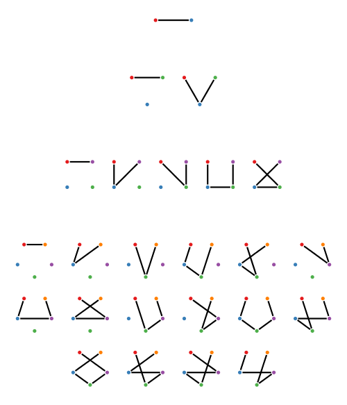
My previous post showed four rows of diagrams, where the 

- start at the top left dot,
- end at the top right dot, and
- never visit any dot more than once.
For a given diagram, we can choose which dots to visit (representing a subset of the dots), and we can visit the chosen dots in any order (a permutation). I will call the resulting things “subset permutations”, although I don’t know if there is some other more accepted term for them.
It’s not necessary to draw subset permutations as paths; it’s just one nice visual representation. If we number the dots from 

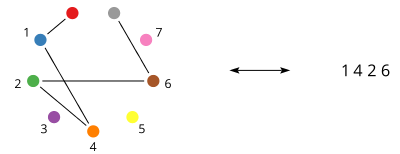
I thought of this idea the other day—of counting the number of “subset permutations”—and wondered how many there are of each size. I half expected it to turn out to be a sequence of numbers that I already knew well, like the Catalan numbers or certain binomial coefficients or something like that. So I was surprised when it turned out to be a sequence of numbers I don’t think I have ever encountered before (although it has certainly been studied by others).
So, how many subset permutations are there of size 


Well, to choose a particular subset permutation of size 


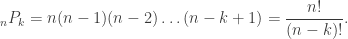
So, in total then, 

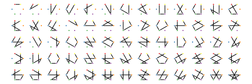
This is already better than just listing all the subset permutations and counting. For example, we can compute that

And sure enough, if we list them all, we get 65 (you’ll just have to take my word that this is all of them, I suppose!):
However, with a little algebra, we can do even better! First, let’s write out the sum for

If we factor 
![\mathit{SP}_n = 1 + n[1 + (n-1) + (n-1)(n-2) + \dots + (n-1)!] = 1 + n \mathit{SP}_{n-1}](https://s0.wp.com/latex.php?latex=%5Cmathit%7BSP%7D_n+%3D+1+%2B+n%5B1+%2B+%28n-1%29+%2B+%28n-1%29%28n-2%29+%2B+%5Cdots+%2B+%28n-1%29%21%5D+%3D+1+%2B+n+%5Cmathit%7BSP%7D_%7Bn-1%7D&bg=ffffff&fg=333333&s=0&c=20201002)
so the subset permutation numbers actually follow a very simple recurrence! To get the
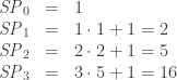
and sure enough, 

A commenter also wondered about the particular order in which I listed subset permutations in my previous post. The short, somewhat disappointing answer is “whatever order came out of the standard library functions I used”. However, there are definitely more interesting things to say about the ordering, and I think I’ll probably write about that in another post.
 we can make
 and
and  . What is the area of the parallelogram?
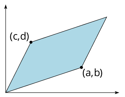


 and want to prove it is a bijection. What can you do?
 is one-to-one, and prove that it is onto.
 and
and  are finite and have the same size, it’s enough to prove either that
  . A proof has to start with a one-to-one (or onto) function
  , and somehow prove that
  defined by
  . Although tricky to come up with, the proof is cute and not too hard to understand once you see it; I think I may write about it in another post!
 such that
  and
and  for all
  and
and  . As we saw in
 be the function that includes the natural numbers in the integers—that is, it acts as the identity on all the natural numbers (i.e. nonnegative integers) and is undefined on negative integers.
  can be the absolute value function. Then
  whenever
  and
and  , for example, the function that sends even
  and odd
  .
. satisfies the condition, but
  defined on the real numbers
  (along with a corresponding
  we have
  . Then applying
  , but because
  . Hence